
What Is a Transformer?
The Transformer is a neural network architecture built to model relationships between words in a sentence. Unlike earlier systems that handled words in strict left-to-right order, the Transformer analyzes all words in a sentence simultaneously — and still determines how each word influences the meaning of every other.
For example, in the sentence “The robot kicked the ball because it was programmed to score,” the word “it” could refer to “robot” or “ball.” The Transformer computes numerical connections between “it” and all other words, then assigns the strongest link to “robot” — based on learned patterns from vast amounts of text.
This article explains the Transformer as it operates on sequences of words — not images, sound, or full documents. We focus only on how it transforms a sentence into a set of context-aware numerical representations, one for each word.
Where Do You See Transformers in Real Life?
Transformers power many everyday tools — not just from big tech companies, but across open-source and commercial AI:
- Autocomplete in messaging apps (e.g., suggesting “coffee?” after you type “Want to grab”)
- Voice assistants (Siri, Alexa) interpreting commands like “Play jazz from the 1960s”
- Open-source models like Llama, Mistral, or BERT used in research, customer support bots, and writing aids
What Came Before Transformers — and Why Did We Need Something New?
Before 2017, most language models were based on Recurrent Neural Networks (RNNs), including improved versions like LSTMs (Long Short-Term Memory) and GRUs (Gated Recurrent Units). These were widely used in speech recognition, machine translation, and early chatbots.
How RNNs Actually Worked
An RNN processes a sentence one token at a time, maintaining a hidden state — a vector that summarizes everything seen so far.
For the sentence “The robot kicked…”, it would:
- Read “The” → update hidden state
- Read “robot” → update hidden state to include “robot”
- Read “kicked” → update again, now encoding “robot kicked”
This hidden state acted as working memory, carrying forward information needed to interpret later words — like remembering that “robot” is an agent, so “it” likely refers back to it.
Why RNNs Hit a Wall
Despite years of use, RNNs faced three hard limits:
- Sequential Bottleneck
Because each step depends on the previous one, RNNs cannot be parallelized. Training on a 50-word sentence requires 50 sequential steps — even on powerful GPUs. A 1,000-word document could take hours per training example. - Vanishing Gradients Over Distance
In practice, RNNs struggled to connect words more than 10–20 tokens apart. If “robot” appeared at position 3 and “it” at position 42, the gradient signal linking them often faded to near zero during training — making correct resolution unreliable. - Fixed Memory Capacity
The hidden state has a fixed size (e.g., 512 numbers). It cannot grow to remember more details. Early words get overwritten or diluted as new ones arrive — like a notepad with only one page.
Researchers added fixes: LSTMs/GRUs improved memory control, and attention mechanisms (circa 2015) let RNN decoders focus on relevant input words. But the core sequential processing remained — limiting speed and scalability.
The Transformer’s Solution
The 2017 paper “Attention Is All You Need” proposed a radical shift: remove recurrence entirely.
Instead of passing a hidden state step by step, the Transformer:
- Treats a sentence (typically up to 512 tokens) as a whole
- Uses self-attention to compute a relevance score between every pair of words, regardless of distance
- Runs all these computations in parallel on GPU cores
This eliminated the sequential bottleneck, allowed reliable connections across hundreds of tokens, and leveraged modern hardware far more efficiently. As a result, Transformers trained 5–10x faster than RNNs on the same data and achieved higher accuracy on tasks like translation and coreference resolution.
The Transformer replaced sequential processing with parallel attention — unlocking faster, deeper, and more contextual language understanding.
What Makes a Transformer Work? The Four Core Components
A Transformer’s power comes from four key parts, applied in sequence:
- Input Embeddings — Turn words into numbers
- Positional Encoding — Add word order
- Multi-Head Self-Attention — Model relationships between words
- Feed-Forward Blocks + Residual Connections + Layer Normalization — Refine and stabilize meaning
These components repeat in stacked layers (often 6 to 12 times), each deepening the model’s understanding.
From Sentence to Meaning
Imagine you type:
“ The robot kicked the ball because it was programmed to score.”
Your Goal:
The model should understand “it” refers to “the robot”, not “the ball.”
This sentence enters the Transformer as raw text. What comes out — after several layers — is a refined numerical representation of each word, now aware of its context.
Input Embeddings: Turn Words into Numbers
Neural networks cannot process raw text directly. Instead, each word (or word fragment) must be converted into a list of numbers that the network can understand and learn from. This list is called a dense vector, and it serves as a numerical “portrait” of the word’s meaning — its semantic meaning.
Think of semantic meaning like a person’s profile in a social app: just as “likes hiking, speaks French, works in robotics” tells you something about who they are beyond their name, a word’s vector captures its role and relationships in language. The word “kick” will have a vector closer to “throw” or “hit” than to “sleep” or “dream”, because the model learns these associations from vast amounts of text.

How does this conversion happen?
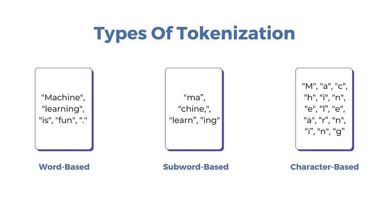
First, a tokenizer — a preprocessing tool built into the model — breaks the input sentence into smaller units called tokens. These tokens can be whole words (“robot”), parts of words (“un”, “do”, “able”), or even punctuation. The choice depends on the tokenizer’s design and the language’s structure.
Each token is then assigned a unique integer ID, known as input_ids. For example, in a given model, “robot” might be ID 4281, “kicked” ID 9032, and so on.
These IDs are not arbitrary labels — they act as addresses that point to specific rows in a large, trainable table called the embedding matrix. This matrix has dimensions vocab_size × d_model:
- vocab_size is the total number of distinct tokens the model was trained to recognize (e.g., 20,000). This vocabulary is fixed during training and belongs to the model itself, not the user or the dataset alone — it’s built from the text data the model originally learned on.
- d_model is the number of values (or dimensions) used to represent each token. If d_model = 512, then every token is described by a list of 512 numbers.
So, when the model sees the token ID for “robot”, it looks up the 4281st row in this matrix and retrieves a 512-number vector that stands for “robot” in its internal language.
This step gives every token a rich numerical identity — but it still knows nothing about where the word appears in the sentence. That comes next.
Input embeddings translate words into a numerical language the Transformer can learn from — like giving every word a fingerprint made of numbers.
Positional Encoding: Adding Word Order
After converting words into numerical vectors, the model still has no idea about their order in the sentence. Without this, the phrases “robot kicked ball” and “ball kicked robot” would produce identical internal representations — leading to serious misunderstandings. To resolve this, the Transformer adds positional encoding: a structured signal that tells the model where each word appears in the sequence.
But how do we represent position numerically — without overwhelming the model with arbitrary numbers?
The original Transformer paper proposed an solution: use mathematical wave patterns — specifically, sine and cosine functions — to generate position-aware vectors. These functions are smooth, predictable, and, crucially, allow the model to extrapolate to longer sentences than it saw during training.

Here’s the intuition:
Imagine assigning each word a unique “rhythm” based on its position. The first word gets one pattern, the second a slightly shifted version, and so on. Because sine and cosine waves repeat in a structured way, the model can learn relationships like “the word two steps ahead” or “the previous word” just by comparing these rhythms.
For each position in the sentence (e.g., position 1, 2, 3…), the model computes a vector of the same size as the embedding (d_model, e.g., 512). In this vector:
- The values at even-numbered positions (0th, 2nd, 4th, …) come from a sine function.
- The values at odd-numbered positions (1st, 3rd, 5th, …) come from a cosine function.
This alternation ensures that every position gets a distinct, high-dimensional signature that changes smoothly as you move through the sentence.
Note: We call the initial numerical representations input embeddings. Once positional encoding is added, we often refer to them simply as embeddings or token representations. The term “word embeddings” is commonly used in the field to describe these learned semantic vectors.
The final representation for each token is the sum of its semantic embedding and its positional vector. The model then learns to interpret this combined signal — for example: “This vector corresponds to the word ‘kicked,’ and it appears in the second position of the sentence.”
Positional Encoding ensures “dog bites man is not same as “man bites dog.”
Layer Normalization: Keeping Numbers in a Healthy Range
As a Transformer processes a sentence, each word is represented by a list of numbers (for example, 512 numbers if d_model = 512). During training, these numbers can grow very large or shrink very close to zero — especially in deep networks with many layers. When this happens, the learning process becomes unstable: small changes in input cause wildly different outputs, and the model struggles to improve.
To prevent this, the Transformer uses layer normalization — a technique that gently rescales the numbers for each word so they stay in a consistent, manageable range.
Here’s how it works:
Take one word in the sentence — say, “kicked.” Its current representation is a list of 512 numbers. Layer normalization looks only at this list (ignoring other words and other sentences in the batch) and adjusts it so that:
- The average (mean) of the numbers becomes 0
- The spread (standard deviation) of the numbers becomes 1
This process is called standardization, a specific type of normalization that centers and scales data. It’s like adjusting the volume of each instrument in an orchestra so no single one drowns out the others.
But what if the model wants some numbers to stay large or small? To preserve flexibility, layer normalization includes two learnable parameters — often called scale (α) and shift (β). These are numbers the model can adjust during training to reverse or modify the normalization if it helps performance. In other words, the model gets to decide how much normalization it actually needs.
Finally, to avoid mathematical errors, a tiny value called eps (e.g., 0.00001) is added during the calculation. This prevents division by zero when computing the standard deviation — especially important when all numbers in a vector are nearly identical.
Where does the (batch, seq_len, d_model) shape come from?
batch: A group of sentences processed together (e.g., 32 sentences at once).
seq_len: The number of tokens in a sentence (e.g., 10 words).
d_model: The size of each word’s vector (e.g., 512 numbers).
So the full data structure is a 3D block: 32 sentences × 10 words × 512 numbers per word. Layer normalization operates independently on each of the 320 word-vectors, one at a time.
Layer normalization acts like an automatic volume control for each word’s internal representation — keeping learning smooth and stable.
Feed-Forward Block: Letting Each Word Reflect on Its Meaning
Within each Transformer layer, two main components work in sequence:
- Multi-Head Attention (which connects words to each other)
- Feed-Forward Block (which processes each word independently)
After attention updates a word’s representation by considering its neighbors, the feed-forward block gives that word a chance to “think on its own” about what it now means in context.
Think of it like this:
During a team meeting, you first listen to everyone’s opinions (that’s attention). Then, you step aside for a moment to reflect privately on what you’ve heard and refine your own thoughts (that’s the feed-forward block). This private reflection happens separately for every participant — no one else is involved.
Technically, this “reflection” is done by a small two-layer neural network applied to each token’s vector:
# Step 1: Expand the vector to a larger space
x → Linear(d_model → d_ff) → ReLU

# Step 2: Compress it back to original size
→ Dropout → Linear(d_ff → d_model)
Here’s what the numbers mean:
- d_model (e.g., 512) is the size of each word’s vector as it moves through the Transformer.
- d_ff (e.g., 2048) is the size of an intermediate, expanded space — typically 4 times larger than d_model.
Why expand? Because working in a larger space gives the model more “room” to separate and combine ideas. For example, the word “bank” might activate some dimensions for “financial institution” and others for “river edge.” The expanded space lets these meanings be teased apart before being recombined.
After this expansion and processing, the vector is compressed back to d_model dimensions (e.g., 512). This ensures that the output of the feed-forward block has the same shape as its input, so it can be passed smoothly to the next layer — whether that’s another Transformer block or the final prediction step. This consistency is essential for stacking many layers without shape mismatches.
The ReLU function (Rectified Linear Unit) adds a simple but powerful rule: any negative number becomes zero. This introduces non-linearity, allowing the model to learn complex patterns instead of just straight-line relationships.
Multi-Head Attention: Understanding Word Relationships
The Transformer’s core mechanism lets every word determine which other words matter most to it in context. We’ll use this sentence:
“The robot kicked the ball because it was programmed to score.”
Our goal it to help the model link “it” to “robot.”
Step 1: Create Queries, Keys, and Values
From each word’s current embedding, the model generates three vectors:
- Query: What the word seeks (e.g., “it” seeks a programmable entity).
- Key: What the word offers (e.g., “robot” signals it is programmable).
- Value: The actual information the word contributes (e.g., traits like “machine,” “agent”).
These are produced by multiplying the embedding with three learned matrices (W<sub>Q</sub>, W<sub>K</sub>, W<sub>V</sub>).
Step 2: Compute Relevance
For “it,” the model calculates a dot product between its query and every other word’s key.
The dot product — sum of element-wise products — measures alignment. A high value means strong relevance.
Step 3: Normalize with Softmax
All dot products for “it” become raw scores. Softmax converts them into attention weights — positive numbers that sum to 1.
For example: 0.82 for “robot,” 0.06 for “ball,” 0.03 for “programmed,” and small weights for the rest.
The ReLU function (Rectified Linear Unit) adds a simple but powerful rule: any negative number becomes zero. This introduces non-linearity, allowing the model to learn complex patterns instead of just straight-line relationships.
Step 4: Build a Contextual Representation
The new vector for “it” is a weighted sum of all value vectors:
New "it" = (0.82 × Value_robot) + (0.06 × Value_ball) + …Because “robot” dominates, the updated “it” now carries numerical features from “robot.” Context is built through this mixture — not by magic, but by math.
Step 5: Use Multiple Heads in Parallel
Instead of one attention process, the Transformer runs 8 (or more) independent heads at once. Each learns different patterns using its own set of W<sub>Q</sub>, W<sub>K</sub>, W<sub>V</sub>.
Each head produces its own output vector for “it.” These are concatenated and passed through a final linear transformation — a matrix multiplication that maps the combined vector back to d_model dimensions (e.g., 512), ensuring compatibility with the next layer.
Multi-head attention lets every word gather contextual evidence from the entire sentence — through multiple independent lenses — before updating its meaning.
Residual Connections: Preserving Original Information
In every Transformer layer, the output of each major component — multi-head attention and the feed-forward block — is added directly to its original input. This design is called a residual connection.
For example, after the attention mechanism updates the representation of the word “it,” the model computes:
New representation = Attention output + Original input before attentionThis simple addition ensures that the core identity of each word — its initial embedding and positional information — is never lost, even after multiple layers of transformation. At the same time, the model can layer on rich contextual updates.
Residual connections are essential for training deep networks. During backpropagation, gradients can flow backward through the “+ input” path without passing through complex transformations. This prevents the gradients from vanishing, which would otherwise stall learning in deep architectures.
Residual connections guarantee that every word carries its original self forward, even as it absorbs new meaning from context.
Putting It All Together: The Full Flow
Consider the sentence:
“The robot kicked the ball because it was programmed to score.”
Here is the complete sequence of operations inside a Transformer encoder:
- Tokenization: The sentence is split into tokens (“The,” “robot,” “kicked,” …).
- Embedding: Each token becomes a dense vector of size d_model (e.g., 512).
- Positional Encoding: A position-specific vector is added to each embedding to mark word order.
Then, the data passes through N identical layers (typically 6 or 12). Each layer performs:
- Multi-Head Self-Attention → Add residual connection → Apply layer normalization
- Feed-Forward Block → Add residual connection → Apply layer normalization
After the final layer, every token is represented by a context-aware vector — a numerical encoding that reflects not only its own meaning but also its role in the full sentence.
These vectors can now be used for tasks like classification, named entity recognition, or as input to a decoder in sequence-to-sequence models.
The Transformer processes an entire sentence in parallel, refining each word’s meaning through repeated cycles of attention, reflection, and identity-preserving updates.
Final Summary: The Four Pillars
The Transformer’s effectiveness rests on four foundational components:
- Word Embedding: Converts tokens into dense numerical vectors that capture semantic meaning.
- Positional Encoding: Encodes the order of tokens in a sequence, enabling the model to distinguish between different word arrangements.
- Self-Attention: Dynamically models relationships among all words in a sentence, allowing each word to influence and be influenced by others.
- Residual Connections: Preserve the original signal through each layer, ensuring stable training in deep networks.
Together, these mechanisms enable parallel, context-aware language understanding — without relying on sequential recurrence or local convolution.
Unlike traditional models that process words one at a time, the Transformer analyzes the entire sentence simultaneously, capturing how every word shapes the meaning of every othe